Welcome to the OmsCilsam module tutorial!

Schema | Inputs | Testing the module with sample dataset | Scripting usage | Output | Utility-Models | References

In this document we will briefly introduce you the module and provide a general overview on its usage.
Most emphasis will be put in describing input data and how to make a test run using the sample dataset.
For a more scientific approach a reference to relevant papers will be given at the and of the document.

A preview of the module can be found in this couple of JAR files containing a custom version of the JGrassTools framework inclusive of the CI-Slam module:
http://www.mcfoi.it/msccs/thesis/jgt-hortonmachine-0.7.7-SNAPSHOT-C.jar
http://www.mcfoi.it/msccs/thesis/jgt-jgrassgears-0.7.7-SNAPSHOT-C.jar

The uDig Desktop GIS is available from here:
http://udig.refractions.net/download/

The module

The module is an implementation of the Ci-Slam stability model. A model for the evaluation of the proneness to instability of each pixel of a map belonging to a single basin, computed using an infinite slope model affected by hydrological variables. It has been conceptualized by C. Lanni et Alii. (2012): see references at bottom of tutorial.
The output, at the current stage of development, is composed by a set of maps containing the Stability Factor of each cell, one for each Return Time requested.
Each map represents the worst-case based composition of a set of maps computed for a single Return Time (RT) and for the number of simulated rainfall events with different durations (1h, 3h, etc.) requested by the user.
Since the model can also be run for one single Return Time, the final output can consist in just one Safety Factor map (with its .prj file).
For example, an output file named:

SAFETY_FACTOR_HYDROLOGIC_30y_1h3h6h_TOT.asc

represents the result of a simulation run for a RT of 30 years and for three different rainfall durations: 1 hour, 3hours and 6 hours.

!!! WARNING - HIGH LOAD ON MEMORY !!!
The module in the current state of development is designed for speed.
This means that it will require NOT LESS than 1.5GB of RAM for each processed square of 1000x1000 pixels. Consequently expect to need from 2.5GB to 6.0GB of RAM to successfully run the model. The amount is particularly affected by longer rainfall durations while the number of supplied Return Times just increases the overall computation time.

Schema

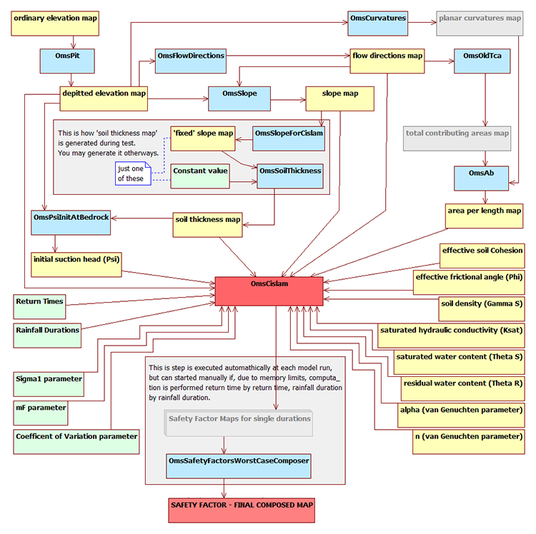
The following schema has been provided to help you get the multiple relations between input and utility-models. A slightly higher resolution one is available here.

Inputs

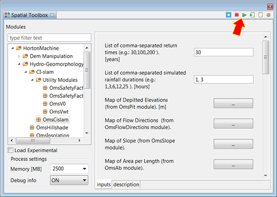
The module can be run using the User Interface provided by the Spatial Toolbox but, due to the number of inputs it is highly recommended to rely on an OMS3 script. A sample one is available inside the input dataset .zip file. See below "Scripting usage" about how to adapt it for your system and run it.

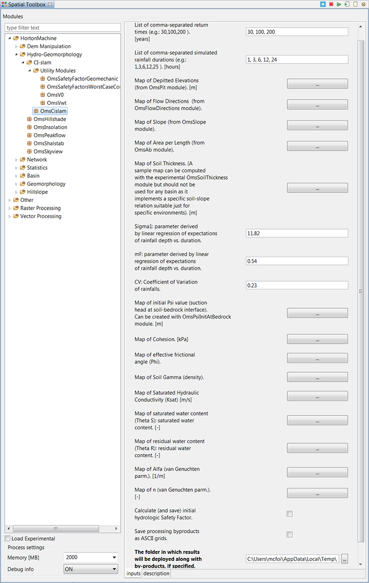
The parameters used for the evaluation of the stability conditions are a good number: a brief description of each is given to follow.

• the comma-separated list of Return Times for which to run the simulation
• the comma-separated list of Rainfall Durations for which to run the simulation

These are the most general inputs of the model and basically control how many times the module will run. In many cases the user will need to perform simulations on return times of 30, 100 and 200 years. On slower machines the user might prefer to split the processing in individual steps so, instead of providing a list of all years all together (e.g.: 30,100,200 ), they might pass one different return time for each run (e.g.: 200).

The simulated rainfall durations are usually provided ALL together (e.g.: 1,3,6,12,24 ). Despite a single Safety Factor map will be computed for each duration, the module also merges all these results into a single worst-case map by selecting the lowest Safety Factor from each map for any cell in the basin.
In the case not enough memory is available in the system, each single simulation can be run alone by submitting one duration at a time (e.g.: 24). In this case the user can compute the total worst-case map using the OmsSafetyFactorsWorstCaseComposer model. This is available among the utility-models that come along with the main one. It accepts a list of rasters (computed for the same return time!) which are then compared to extract the lowest safety factor in each map for any cell.

• the depitted elevation map
• the flow directions map
• the slope map
• the area per length map

This is the "ordinary" set of maps the user should be already familiar with as are the maps that are used to compute most landscape indexes based on topography.
They are usually ESRII ASCII grids bearing the '.asc' extension: files that can so be inspected with any plain text editor.
Actually just the elevation map is required and for that coverage the module prescribes it not to contain pits. This can be obtained with the OmsPit module that takes an elevation map as the only input.

All other maps can be derived from the first, also using some of the other OMS modules available in the JGrassTools.
In the table to follow a workflow is provided that starts from an "ordinary elevation map" to produce the four required maps:

• the soil thickness map

The soil thickness map deserves a specific comment. The model pervasively uses this map to compute important internal parameters like the time required by each cell to develop a perched water table at soil-bedrock interface (saturation) for vertical infiltration (during rainfall). This means that providing a realistic map of soilt thickness is of great importance. For the sole use as an example, the OmsSoilThickness modules is provided (requires checking 'load experimental' to be displayed): this modules derives the soil thickness map using the slope map. Read the module description for details.

• the Sigma1 parameter
• the mF parameter
• the Coefficent of Variation parameter

All these are parameters that are computed from the statistical analysis of rainfalls history of the investigated basin. The default suggested values available in the Spatial Toolbox windows are right just for running the test with the default dataset. Needless to say: they PROBABILY HAVE NO MEANING for your basin. Replace them with proper ones when running the module on your data!

• the map of initial suction head (Psi) at soil-bedrock interface
• the map of effective soil Cohesion
• the map of effective frictional angle (Phi)
• the map of soil density (Gamma S)
• the map of saturated hydraulic conductivity (Ksat)
• the map of saturated water content (Theta S)
• the map of residual water content (Theta R)
• the map of alpha (van Genuchten parameter)
• the map of n (van Genuchten parameter)

This last big set of maps covers the wide range of parameters that define the geomechanic and hydrologic features of the soil of the basin.
Those maps that should be possible to insert as single constant values to be used over all the basin (soil thickness, psi, cohesion, ecc) have to be provided in any case as maps. Other modules such as OmsMapcalc can be useful to cover such tasks.

Testing the module with sample dataset

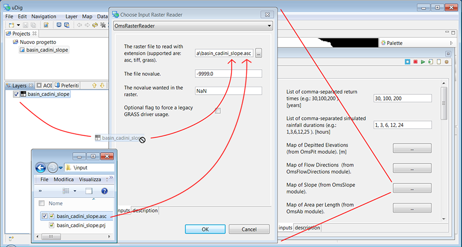
In the zipped sample dataset, one single map for each input is available. The file names define the purpose of each map.

The zip file must be extracted into a path that should NOT contain whitespaces (this is specially true for Windows). Then each map should be set as the input of the relative parameter. This can be done by dragging the files from their folder directly on the the Spatial Toolbox. If any map is already loaded in uDig, also dragging from the layer-list is a possibility.

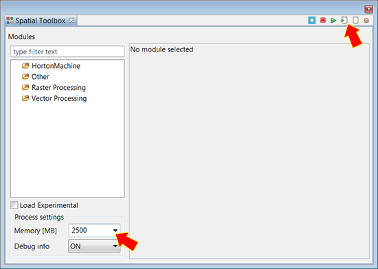
To run the test we suggest to provide a single value for Return Times: 30
This will minimize computation times.

To extabilish a low memory requirement, we also suggest to input just two values for Rainfall Durations: 1,3
In this way the Memory [MB] for the process can be set to a value of 2500

Finally, it is important to specify an Output Folder (despite the default temp dir is suggested): in that location all produced files will be deployed.
Note that, if "Save processing byproducts as ASCII grids." is checked, the output files can reach a total volume of more than 2GB.

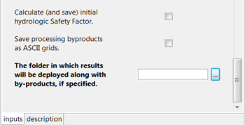
Upon request (checking the relevant box) also the optional initial hydrologic Safety Factor map can be computed: a safety factor controlled by hydrological parameters but not considering rainfalls.

To start the test just press the "play" button and follow the progresses in the uDig's console window.

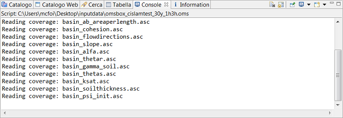
The tool should compute for 2-3 minutes while displaying progresses in the Console:

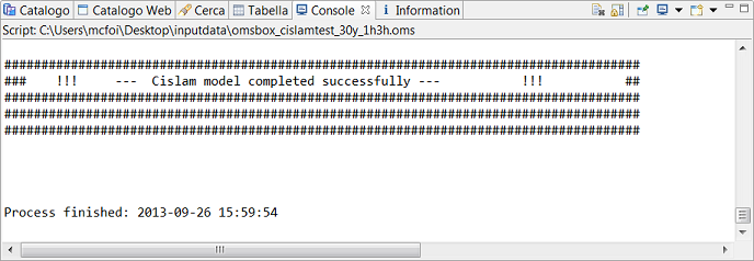
and complete by returning the following message:

In case the tool runs out of memory and an "Out Of Memory" exception is thrown, you should get an error like this one:

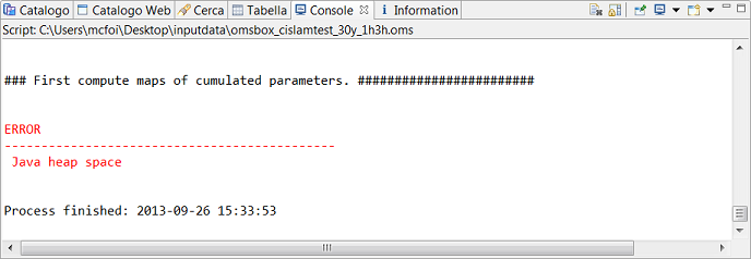
In this case you can either increase the memory reserved for the process (if you have it) or try splitting it in single Return Times and single Rainfall Durations, to then resort to the OmsSafetyFactorsWorstCaseComposer model to compute the total map for each return time.

Scripting usage

The test can be run also using a script. This approach has the advantage of saving from the tedius activity of specifying all inputs every time a new run is needed and most/many of the involved maps are the same.

A sample script is provided in the zip containing the test input data: here is its content:

def simulation = new oms3.SimBuilder(logging:'OFF').sim(name:'OmsCislam') {

model {

components {
'cislam0' 'cislam'
'rasterreader1' 'rasterreader'
'rasterreader2' 'rasterreader'
'rasterreader3' 'rasterreader'
'rasterreader4' 'rasterreader'
'rasterreader5' 'rasterreader'
'rasterreader6' 'rasterreader'
'rasterreader7' 'rasterreader'
'rasterreader8' 'rasterreader'
'rasterreader9' 'rasterreader'
'rasterreader10' 'rasterreader'
'rasterreader11' 'rasterreader'
'rasterreader12' 'rasterreader'
'rasterreader13' 'rasterreader'
'rasterreader14' 'rasterreader'
}

parameter {
'cislam0.pReturnTimes' '30'
'cislam0.pRainfallDurations' '1, 3'
'rasterreader1.file' 'C:/Users/mcfoi/Desktop/inputdata/basin_depitted_dem.asc'
'rasterreader1.fileNovalue' '-9999.0'
'rasterreader1.geodataNovalue' 'NaN'
'rasterreader1.doLegacyGrass' 'false'
'rasterreader2.file' 'C:/Users/mcfoi/Desktop/inputdata/basin_flowdirections.asc'
'rasterreader2.fileNovalue' '-9999.0'
'rasterreader2.geodataNovalue' 'NaN'
'rasterreader2.doLegacyGrass' 'false'
'rasterreader3.file' 'C:/Users/mcfoi/Desktop/inputdata/basin_slope.asc'
'rasterreader3.fileNovalue' '-9999.0'
'rasterreader3.geodataNovalue' 'NaN'
'rasterreader3.doLegacyGrass' 'false'
'rasterreader4.file' 'C:/Users/mcfoi/Desktop/inputdata/basin_ab_areaperlength.asc'
'rasterreader4.fileNovalue' '-9999.0'
'rasterreader4.geodataNovalue' 'NaN'
'rasterreader4.doLegacyGrass' 'false'
'rasterreader5.file' 'C:/Users/mcfoi/Desktop/inputdata/basin_soilthickness.asc'
'rasterreader5.fileNovalue' '-9999.0'
'rasterreader5.geodataNovalue' 'NaN'
'rasterreader5.doLegacyGrass' 'false'
'cislam0.pSigma1' '11.82'
'cislam0.pmF' '0.54'
'cislam0.pCV' '0.23'
'rasterreader6.file' 'C:/Users/mcfoi/Desktop/inputdata/basin_psi_init.asc'
'rasterreader6.fileNovalue' '-9999.0'
'rasterreader6.geodataNovalue' 'NaN'
'rasterreader6.doLegacyGrass' 'false'
'rasterreader7.file' 'C:/Users/mcfoi/Desktop/inputdata/basin_cohesion.asc'
'rasterreader7.fileNovalue' '-9999.0'
'rasterreader7.geodataNovalue' 'NaN'
'rasterreader7.doLegacyGrass' 'false'
'rasterreader8.file' 'C:/Users/mcfoi/Desktop/inputdata/basin_phi.asc'
'rasterreader8.fileNovalue' '-9999.0'
'rasterreader8.geodataNovalue' 'NaN'
'rasterreader8.doLegacyGrass' 'false'
'rasterreader9.file' 'C:/Users/mcfoi/Desktop/inputdata/basin_gamma_soil.asc'
'rasterreader9.fileNovalue' '-9999.0'
'rasterreader9.geodataNovalue' 'NaN'
'rasterreader9.doLegacyGrass' 'false'
'rasterreader10.file' 'C:/Users/mcfoi/Desktop/inputdata/basin_ksat.asc'
'rasterreader10.fileNovalue' '-9999.0'
'rasterreader10.geodataNovalue' 'NaN'
'rasterreader10.doLegacyGrass' 'false'
'rasterreader11.file' 'C:/Users/mcfoi/Desktop/inputdata/basin_thetas.asc'
'rasterreader11.fileNovalue' '-9999.0'
'rasterreader11.geodataNovalue' 'NaN'
'rasterreader11.doLegacyGrass' 'false'
'rasterreader12.file' 'C:/Users/mcfoi/Desktop/inputdata/basin_thetar.asc'
'rasterreader12.fileNovalue' '-9999.0'
'rasterreader12.geodataNovalue' 'NaN'
'rasterreader12.doLegacyGrass' 'false'
'rasterreader13.file' 'C:/Users/mcfoi/Desktop/inputdata/basin_alfa.asc'
'rasterreader13.fileNovalue' '-9999.0'
'rasterreader13.geodataNovalue' 'NaN'
'rasterreader13.doLegacyGrass' 'false'
'rasterreader14.file' 'C:/Users/mcfoi/Desktop/inputdata/basin_n.asc'
'rasterreader14.fileNovalue' '-9999.0'
'rasterreader14.geodataNovalue' 'NaN'
'rasterreader14.doLegacyGrass' 'false'
'cislam0.doCalculateInitialSafetyFactor' 'true'
'cislam0.doSaveByProducts' 'true'
'cislam0.pOutFolder' 'C:/Users/mcfoi/Desktop/OUTPUT/'
}

connect {
'rasterreader1.outRaster' 'cislam0.inPit'
'rasterreader2.outRaster' 'cislam0.inFlow'
'rasterreader3.outRaster' 'cislam0.inSlope'
'rasterreader4.outRaster' 'cislam0.inAb'
'rasterreader5.outRaster' 'cislam0.inSoilThickness'
'rasterreader6.outRaster' 'cislam0.inPsiInitAtBedrock'
'rasterreader7.outRaster' 'cislam0.inCohesion'
'rasterreader8.outRaster' 'cislam0.inPhi'
'rasterreader9.outRaster' 'cislam0.inGammaSoil'
'rasterreader10.outRaster' 'cislam0.inKsat'
'rasterreader11.outRaster' 'cislam0.inTheta_s'
'rasterreader12.outRaster' 'cislam0.inTheta_r'
'rasterreader13.outRaster' 'cislam0.inAlfaVanGen'
'rasterreader14.outRaster' 'cislam0.inNVanGen'
}

}

}
result = simulation.run();

println " "

To be used, the script needs to be adapted to your system. Specifically two things have to be updated:

- local path of input data

Code parts like 'C:/Users/mcfoi/Desktop/inputdata/basin_pit.asc' require you to replace the path with the right one pointing to where you extracted the test dataset. Please avoid folder names containing whitespaces!

- location of output folder

The string 'C:/Users/mcfoi/Desktop/OUTPUT/' should also be fixed.

Note that the FORWARD SLASH " / " must ALWAYS be used ALSO in Windows paths. Otherwise the module will fail on launch complaing that an unexpected '\' was found.

Clearly also Return Times, Rainfall Durations, as well as Sigma1, mF and Coefficient of Variation have to be adapted to your input.

Do not forget to consider whether you need to have the initial Safety Factor to be computed and byproducts exported to files: if not the case set to 'false' the relative parameters.

Once the script is ready, it can be run directly from the action bar of the uDig's Spatial Toolbox, without the need of even finding the OmsCilsam module in the tree menu.. ..but do not forget to set the Memory value before loading the script!

Output

The output file is usually composed by one or more maps of the Safety Factor, one for each Return Time requested.

In the case of the test, run for a Return Time of 30 years and with two Rainfall Durations (1h an 3h), the result will be a single ESRI ASCII grid (with its .prj file), located in the specified output folder and named:

SAFETY_FACTOR_HYDROLOGIC_30y_1h3h_TOT.asc

Its cell are filled with a value representing the Safety Factor for the specific area.

• <1 : unstable cell
• >1 : stable cell
• -9999 : no-value area

Utility-Models

The main module is delivered along with a set of utility-modules. These are all sub components of the main module and are used internally during each of its run. Therfore most of these are exposed more for comprehension than for actual use. They are expected to be run to produce some by-products for study as most of these outputs cannot be feed back in the main workflow.

Here is the list of modules ordered by involvement in the main workflow:

References